1D vs 2D domain decomposition for parallel execution on regular grids
This post is a brief summary of the paper on parallel computing with regular grids (link).
It describes the advantage of 3D domain decomposition over 1D or 2D domain decomposition for distributed memory computing with a stencil code because of the better surface to volume ratio (computation to communication ratio).
Many simulations are performed on a regular 3D grid. Seismic wave propagation, fluid flow or grain growth are a view examples, which are computed on regular grids. It is often referred to stencil codes because a stencil is applied to compute the next state in time for each grid cell. 1D and 2D domains are favorable, because of small stencils and small memory foot prints, which leads to a fast computation and less cache misses. Unfortunately, many phenomena need to be investigated in 3D. Lets stay in the 2D world till the end because it is possible explain the effects on speedup and efficiency already in 2D.
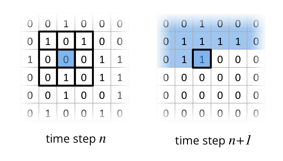
One very accessible example for a stencil code on a 2D grid is Conway’s Game of Life, where a cell is either alive 1 or dead 0. Four simple rules determine if a cell dies, starts to live ;-) or stays in the same state based on a 9-point stencil as depicted in the following figure.

In this example I have one 2D grid for the current time step $n$ and one for the next time step $n+1$. The field with time step n contains a initial state, which is randomly filled with alive (1) and dead (0) cells. To compute the state of all cells in the grid for time step $n+1$, the 9-point stencil has to be applied for all cells in in time step $n$. The following figure depicts the two fields (time step $n$ and $n+1$) and shows the application of the 9-point stencil on a cell. Already processed cells in time step $n+1$ are colored in blue.
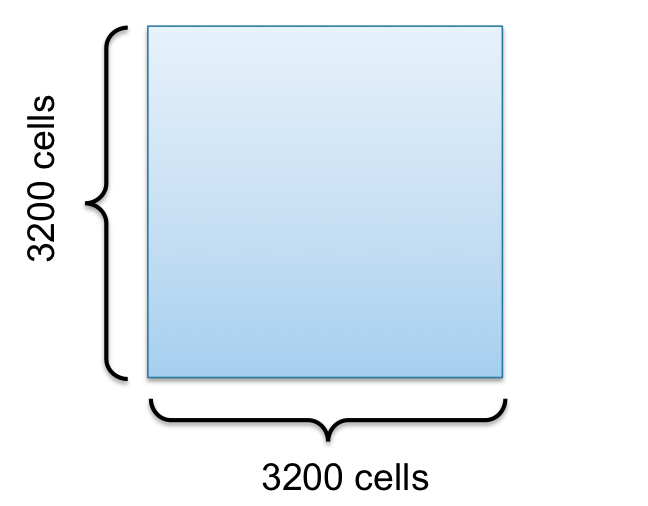
Now lets take a look at a 2D grid consisting of $3200\times3200$ cells to get into domain decomposition for Conway’s Game of Life 9-point stencil example.
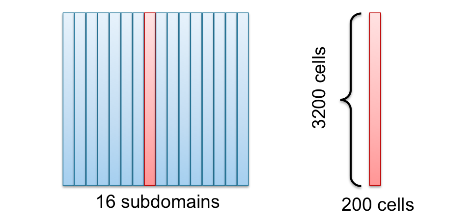
I use 16 CPU cores to speedup the computation, such that I cut the domain along the $x$ axis into 16 subdomains as you can see in the following figure. One domain (red) is picked out to show the size of the domains.
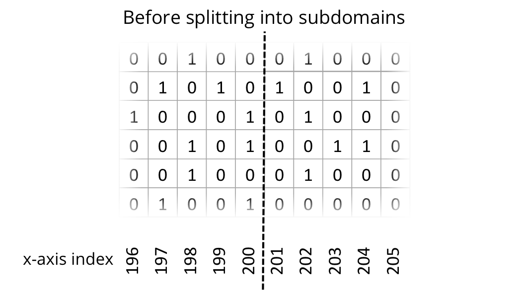
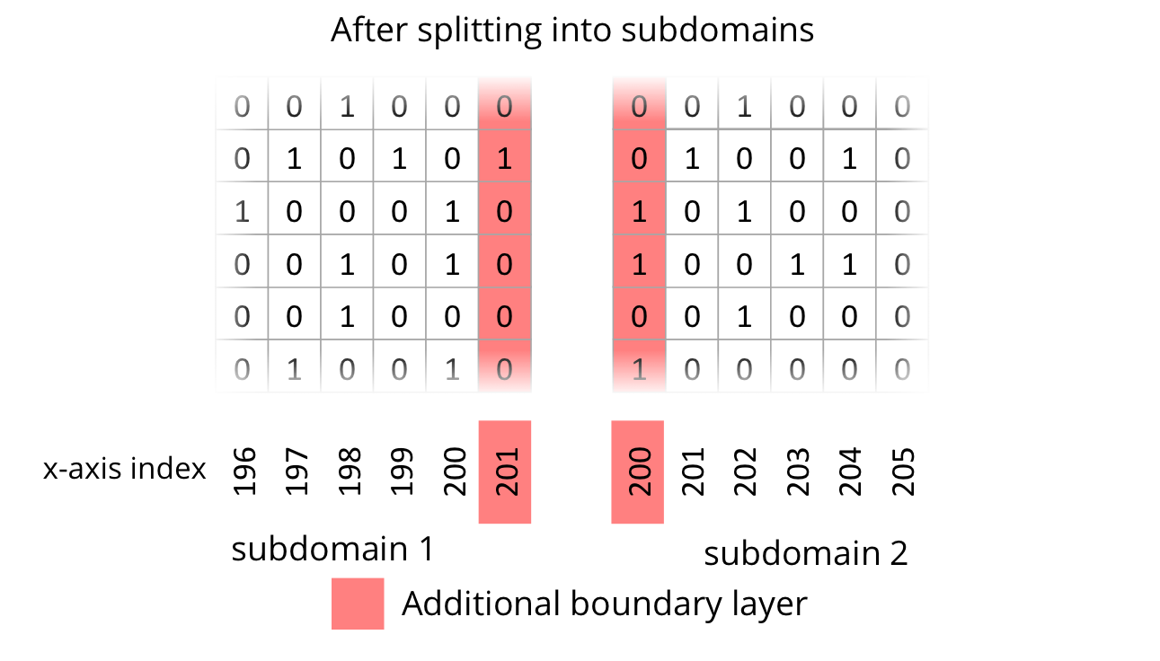
In order to compute one subdomain independently on one processor, it is necessary to introduce one additional line of cells at the cutting edge. In other words, a boundary layer or ghost layer has to be introduced. The following two figures depict the state of the uncut domain and the state after cutting into subdomains with additional ghost layers.
The final part is to update the ghost cells after each time step, which requires communication. Now communication is the dark side of computing. Its the reason for the caches on the CPUs. If you want to utilize a cluster of over 10.000 CPU cores, communication over a network is necessary, such that the boundary exchange or boundary updates are performance critical.
To estimate the performance of a $3200\times 3200$ cells domain lets assume the computation of one 9-point stencil $t_s$ requires 1 time unit and the communication time$t_c$ of one cell requires also 1 time unit, then the runtime $T_{s}$ would look something like this for the sequential case with 1000 time steps.
$T_{s}=3200^2 \cdot t_s \cdot 1000$.
The parallel runtime with 16 cores $T_p$ is
$T_{p}=(3200 \cdot 200 \cdot t_s + 3200 \cdot 2 \cdot t_c)\cdot 1000$.
The speedup $S$ would be
$S=\frac{T_s}{T_p}=\frac{3200^2 \cdot t_s \cdot 1000}{(3200 \cdot 200 \cdot t_s + 3200 \cdot 2 \cdot t_c)\cdot 1000}=\frac{3200\cdot t_s}{200\cdot t_s + 2 \cdot t_c}=\frac{3200}{202}\approx 15.84$,
which sounds not bad. Now lets increase the cores to 128.
$S=\frac{T_s}{T_p}=\frac{3200^2 \cdot t_s \cdot 1000}{(3200 \cdot 25 \cdot t_s + 3200 \cdot 2 \cdot t_c)\cdot 1000}=\frac{3200\cdot t_s}{25\cdot t_s + 2 \cdot t_c}=\frac{3200}{27}\approx 118.52$
A Speedup of about 119 is also nice with 128 CPU cores. Lets go to the end of the line with 3200 CPU cores.
$S=\frac{T_s}{T_p}=\frac{3200^2 \cdot t_s \cdot 1000}{(3200 \cdot 1 \cdot t_s + 3200 \cdot 2 \cdot t_c)\cdot 1000}=\frac{3200\cdot t_s}{1 \cdot t_s + 2 \cdot t_c}=\frac{3200}{3}\approx 1066.67$
This now looks a little weird. 3200 Cores create a speedup of about 1067. What happened with the other cores. Are they sitting idle? Yes, communication is the bottleneck. This example and the performance model are simple and some assumptions are made, such that I strongly advice to make measurements before you conduct development. If your Measurement show the same or similar scaling behavior, you should consider multi dimensional decomposition as one option. One step to optimize would be to hide communication as much as possible but to reduce the communication to a minimum tackles the problem directly.
To reduce communication, the cutting surface (red cells from the last figure) have to be reduced by cutting the domain in squares instead of salami slices as shown in the following picture.
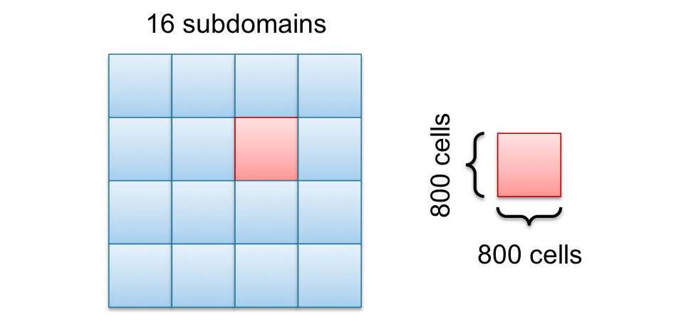
The main difference between the square in the last picture and the salami slices in the earlier picture is not the number of cells inside the domain, its the cutting surface. The square has a cutting line of $800\times 4 = 3200$ and the salami slice has $3200 \times 2 = 6400$ cells, which is the double amount. This will not affect the speedup much for small numbers of CPU cores but for large numbers.
Lets see what happens for 3200 cores.
$S=\frac{T_s}{T_p}=\frac{3200^2 \cdot t_s \cdot 1000}{(3200 \cdot t_s +\frac{3200}{\sqrt{3200}} \cdot 4 \cdot t_c)\cdot 1000}=\frac{3200\cdot t_s}{1 \cdot t_s + \frac{4}{\sqrt{3200}}\cdot t_c}=\frac{3200}{1.07}\approx 2988.67$
Now this looks much nicer with a speedup of about 2989 instead of 1067 with 3200 CPU cores.
The scaling behavior between 1D decomposition 2D decomposition is significantly different. If you have a 3D volume, the decomposition dimension matters even more.