• Some Slides
  • Customers
    • Repair Shop
    • Saar
    • Sopp
  • About Me

Alexander Vondrous

echo "Hello Word!"

Allgemein

Benefits of “Row Recycling”

15. March 2021 by sasa Leave a Comment

TLDR

Make updates, don’t delete rows just to insert them with small changes.

The Crime Scene

In the shadows of the night, a batch job starts his task at 2 am to clean data. A table with millions of entries and more columns then healthy for any developer gets queried for new entries of the last working day. Each cleaning step comes in chunks of 1 to 10 rows. From here on out, there are three different ways a chunk of rows can develop. Either the number of rows in a chunk increases, stays as it is or decreases. In any way, the content is slightly modified. This batch jobs takes about 2 to 3 hours to complete processing all the chunks sequentially.

The Culprit

To process all chunks, all changed rows of the last working day get fetched and processing starts:

  1. Start Transaction
  2. Get all rows of a chunk
  3. Delete all rows of the chunk from the database
  4. Modify the row content and row count
  5. Insert the modified rows of the chunk into the database
  6. End Transaction

The delete-modify-insert pattern works well for a certain size of table but can get slow as soon as the content of the table gets out of hand. An update could be faster than delete-modify-insert. 

Old developers wisdom: Make measurements, especially if in doubt.

Delete and insert operations are expensive because the index has to be updated. It also depends strongly on the tables configuration and database settings. Some databases can handle it very well but in this case it was the reason for a moderate performance.

One Solution: Row Recycling

To optimize chunk processing, keep the rows of a chunk in the database to the moment, when it is clear, how the new chunks look like in terms of row count and content. Three scenarios are possible:

  1. number of rows stays the same
  2. number of rows decreases
  3. number of rows increases

In any case, row content is slightly modified. With that knowledge, it is possible to create a model to understand possible performance benefits. Lets get the hands dirty. The property of interest is speedup $S$, which we could gain from recycling rows to get rid of the delete-modify-insert schema. Speedup is defined as the time the old program (old: delete-modify-insert) takes $T_{o}$ by the time the new program (new: lets call it recycle) $T_{n}$ takes. 

$S = \frac{T_{o}}{T_{n}}$

The time a delete-modify-insert $T_{o}$ takes, consists of the time $t_d$ it takes to delete one of $n$ elements and the time $t_i$ to insert one of $m$ elements.

Wait a minute: Where is the time to fetch, modify and send the data?

There are several reasons to remove those considerations. The very first and obvious reason is, the “recycling speedup” I want to show looks much better clearer ;-). Another reason is to keep the model simple for this post. The most reasonable reason is to neglect the latency bound operation becaues the database and batch process are on the same machine. Its an easy task to add more and more reality/complexity to the model which would make a really long post with dozens of parameters. Simplicity is good because one can use available tools at hand (e.g. Mathematica, …) to analyze certain aspects of reality, without the need to develop a professional simulator, which is fun though.

Now lets get the equations going and define $T_{o}$

$T_{o} = n\cdot t_d + m\cdot{} t_i$

The situation for $T_{n}$ is a little bit more complex but still managable, because the three cases (row count increases, stays and decreases) from above are used. The time to update a row is $t_u$.

$T_{n} = \begin{cases} (n-m) \cdot{} t_d & + & m\cdot{}t_u, & \text{if $m<n$} \\
 & & m\cdot{}t_u, & \text{if $m=n$} \\
(m-n) \cdot{} t_i & + & n \cdot{}t_u, & \text{if $m>n$} \end{cases}$

I simplified the equation (some Voodoo) with one Assumption: The time it takes to delete a row is the same time it takes to insert a row. This is heavy and it was true for that “crime”. Imagine the length and width of the database table to get such performance behaviour.

$T_n = |n-m|\cdot{}t_d + \text{min($m,n$)}\cdot{}t_u$

Lets put everything into the cooking pot and determine the Speedup.

$S = \frac{T_{o}}{T_{n}} = \frac{n\cdot t_d + m\cdot{} t_d}{|n-m|\cdot{}t_d + \text{min($m,n$)}\cdot{}t_u} = \frac{n+m}{|n-m| + \text{min($m,n$)}\frac{t_u}{t_d}}$

To understand a little bit better, what this means, lets take another perspective on this equation with surface plots. The x-axis is $n$ and the y-axis is $m$. The quotient $\frac{t_u}{t_d}$ is set to 1.0 (update and delete time is equal). The z-axis is representing the Speedup $S$. Here the Mathematica line:

Plot3D[(x+y)/(Abs[x-y]+Min[x,y]*1), {x, 0, 10}, {y, 0, 10}]
The plot is symmetrical to the first bisector and has a maximum speedup of about 2.

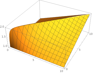
Now this looks good. In the worst case the speedup of row recycling is as good as without recycling (delete-insert). Things start to look even better if the time for an update is smaller than for a delete/insert. Lets assume an update is 10 times faster than a delete.

Plot3D[(x+y)/(Abs[x-y]+Min[x,y]*0.1), {x, 0, 10}, {y, 0, 10}]
The same as earlier but the maximum speedup is around 15.

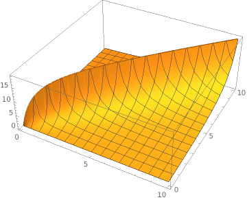
Now this shark fin is a good result. Lets push things one order of magnitude and assume an update is 100 times faster than a delete/insert.

Plot3D[(x+y)/(Abs[x-y]+Min[x,y]*0.01), {x, 0, 10}, {y, 0, 10}]
Wow the result is, that one has to increase the bounding box 😉.

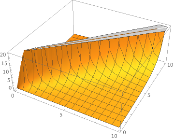
Ok ok but what happens if the time of an update is 10 times slower than an delete/insert?

Plot3D[(x+y)/(Abs[x-y]+Min[x,y]*10), {x, 0, 10}, {y, 0, 10}]
The surface is also symmetrical along the first bisctor and in the worst case, we are about 10 times slower than delete-insert.

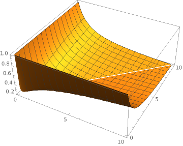
This does not look very good but every coin has two sides. Its somehow clear, if an update takes 10 times the time of a delete or insert, that the update centric approach ist slower. Heads up. This is not the end. Something interesting happens if the time for an update is two times the time of a delete/insert.

Plot3D[(x+y)/(Abs[x-y]+Min[x,y]*2.0), {x, 0, 10}, {y, 0, 10}]
Its a plane 🤨.

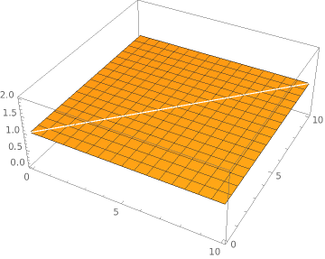
This is very interesting, since there is no speedup at all. This shows, that it is possible that an optimization can have no speedup at all. Imagine the confusion analysing such behaviour after a performance optimization.

All in all its imperative to understand and proof performance bottlenecks before conducting an optimization like “row recycling”. The delete-insert method has benefits if the update takes way to long but the update is clearly benefitial if the update time is equal to the delete/insert time for this use case.

There are more things to explain around this use case, more things to discuss and more things to analyse. If you like, let me know.

Posted in: Allgemein Tagged: database, optimization, performance modelling

Scary Halloween Lights

28. October 2018 by sasa Leave a Comment

1st test of the “scary light barrier”:

The flickering is not on purpose but it looks scary.

Posted in: Allgemein

Indication to Celebrate Birth as Most Important Birthday

29. August 2018 by sasa 3 Comments

The e.g. 30th birthday is celebrated with more attention than the 27th birthday. Why is this so? The reason is the zero after the three or in mathematical terms the multiple of ten (your daily numeral system with base 10). As a computer affine guy I celebrate the 32nd birthday even more because it has a lot more zeros, at least in the binary, octal, hexadezimal and duotrigesimal (base 32) numeral systems. The small and not so unimportant question appeared.

Which birthday has to be celebrated the most?

This gives me the opportunity to use one of my favorite computation methods: Brute Force. I like to use brute force algorithms because of their simplicity. There are no gradients I have to follow, no clever selection of choices, no neural gas and no discussion about the runtime order because brute force algorithms perform badly. A big plus is, that you scan the whole parameter space without exception.

Now back to the task: Which is the birthday with the most zeros in “all” number systems? Actually I only use the number systems from 2 to 128 because no human according to Wikipedia got older than 122 years and I like numbers, which are two to the power of a natural number.

Lets establish the solution step by step and than perform some induction programming. The idea is to find a simple mathematical rule, which gives us the number of zeros. Lets start with the binary system. The following numbers are interesting for our solution:

Base 2 Numeral System Short Decimal Representation Decimal Representation Number of Zeros
10 $2^1$ 2 1
100 $2^2$ 4 2
1000 $2^3$ 8 3
10000 $2^4$ 16 4
100000 $2^5$ 32 5
1000000 $2^6$ 64 6
10000000 $2^7$ 128 7
100000000 $2^8$ 256 8

One could assume, to go through each base $b$ with the exponent $e$ and the exponent gives us the number of zeros. This has a caveat which is shown in the following table for the numeral system with base three:

Base 3 Numeral System Short Decimal Representation Decimal Representation Number of Zeros
10 $1 \cdot 3^1$ 3 1
20 $2 \cdot 3^1$ 6 1
100 $1 \cdot 3^2$ 9 2
200 $2 \cdot 3^2$ 18 2
1000 $1 \cdot 3^3$ 27 3
2000 $2 \cdot 3^3$ 54 3
10000 $1 \cdot 3^4$ 81 4
20000 $2 \cdot 3^4$ 162 4

This looks like a better solution with $n$ from 1 to $b-1$ times $b^e$. The caveat here is, that $110_3$, $120_3$, $210_3$ etc. are missing in the list. 

Another problem with the decimal system we live in. It does not explain if we celebrate the $101$ birthday more then the 10th birthday? Lets keep it simple and say: Each zero counts, no matter of its place in the number.

Because the very simple mathematical solutions do not get the results I want, I would have to switch on my brain to figure a clever way to find the solution. Because thinking is difficult, I start programming ;-)

The idea is to represent a year in all number systems from base 2 to base 128 (127 systems) and then to count the zeros. Do this for all years from 0 128. Et Voila. To do this a new Python script is born:

Gist: https://gist.github.com/Threadmonkey/bf07ee6af7134d8b5b90cabe595f3778

As you can guess, birth at year 0 has in ‘all’ numeral systems a zero, which makes it the winner by far. Here a chart with the number of zeros on the y-axis and the years on the x-axis.

To see a little bit more details, here without the outlier.

Conclusion

  • Celebrate your birth as much as you can
  • The older you get the better/harder you have to celebrate/party
  • The 72nd birthday is the new 50th birthday
  • The 72nd birthday is even the new 100th birthday

I hope you had fun reading. If there is a broader interest in this topic, I would invest more time on a more detailed investigation. Let me know.

Posted in: Allgemein Tagged: birth, birthday, celebrate, party, why

PhD Survival Kit

23. August 2015 by sasa Leave a Comment

You have decided to get a PhD. OK but I cannot let you do it without giving you a few life saving instructions in order to survive. Most human beings do not know what it means to get a PhD. You have to say goodbye to about 18 years of protection by the syllabus mommy. You leave the warm home, where teachers and professors tell you what to learn and what to do.

Welcome to the wild side. Its like becoming a member of a tribe with crazy rites, a chief (professor), subordinates (post docs), sub-subordinates (PhD students), sub-sub-subordinates (students) and handicrafts (structured paper stacking, reading multi color layered white board paintings, dealing with different types of deadlines, …). Because life in the wild is tough here a list of websites you should use during your PhD to adapt to the new circumstances.

Phd Comics (Jorge Cham)
At the beginning of your thesis you will laugh, later you will use it as a source for compassion ;-).
http://phdcomics.com/comics.php

XKCD (Randall Munroe)
If you need something else to think about with relation to maths, technology, childish or grown-up curiosity you will enjoy XKCD.
http://www.xkcd.com
(If you are not able to enjoy it: http://www.explainxkcd.com)

The magic button
If nothing works, this button will also not work. At least you will feel a little bit better.
http://make-everything-ok.com

Correlation?
Some correlations are just not as true as necessary for a publication.
http://www.tylervigen.com

Paper generator
Its true, there is a generator for papers, which works. Unfortunately you have to submit often till it gets accepted.
http://pdos.csail.mit.edu/scigen/

Nobel prize
If you cannot get the real one, you can at least bring glory and honor to your institute with the ig Nobel prize.
http://www.improbable.com/ig/

List of not obvious (techy) procrastination sites
http://dilbert.com/ (ok this one is obvious)
http://thecodinglove.com/
http://devopsreactions.tumblr.com/
https://devhumor.com/

A little bit more useful procrastination sites
http://www.ted.com/
http://99u.com/

I wish you well and hope to see you in some of the dance your PhD videos.
http://gonzolabs.org/dance/

Posted in: Allgemein Tagged: phd, procrastination, survival kit

Ready, Steady, GOOOOO

11. August 2015 by sasa Leave a Comment

Traffic jams and rush hours reduce my free time, which I can spend with more meaningful activities. Usually I use the commute to come down from work and to switch into private mode. Unfortunately I do not need an hour to arrive in the private world, such that I waste a lot of time in the car. Even the best podcasts are sometimes of no use to bridge the time. In order to reduce the commute time from my office to my home, I tried experimentally to figure out which departure time is the best. Beside the desired sampling rate and a long observation period, I am lazy and I forget to make notes. After a week the experiments felt fuzzy and the way of solving the problem did not satisfy the little nerdiness I carry with me but I got the best case and worst case timings:

Travel distance:                50 km
Best case (moderate speed):     35 minutes
Best case (pedal to the metal): 30 minutes
Worst case:                     60 minutes

What do humans in the 21st century use to estimate the travel time? Google maps! OK thats the way to go. The nice thing is, that google maps is able to take the current traffic situation into account. I can let the computer do the nasty work of taking notes.

Bildschirmfoto 2015-08-11 um 22.06.05

Within 80 lines of Java code (with empty lines ;-), the google maps API is queried every minute and the result is stored in a file. After about $3.5$ weeks of data acquisition a bash script extracts and groups the estimated travel time for each day of the week into a single file. One data point consists of the time and estimated travel time pair: “HH-MM-SS : estimated travel time”. Up to 4 data points of each minute made the visualization messy. To reduce the number of data points a python script computes the mean value for each minute. Finally D3 javascript is used to visualize the data as you can see if you click on one of the following weekdays.

Monday, Tuesday, Wednesday, Thursday, Friday, Saturday, Sunday

Between 1 am  and 5 am google does not deliver travel time estimations or the more probable explanation is, that google knows about a stargate nearby, which opens from 1 am to 5 am. Beside the things google knows, the interesting parts for me are the rush hour peaks around 5 pm. On Monday there is surprisingly no peak. Maybe the measurement period of about $3.5$ weeks was to short. On Tuesday and Wednesday the peaks are after 5 pm and on Thursday and Friday the peaks are shifted towards 4pm. Surprisingly a 12 o’clock peak occurs on saturday. A colleague called it “the Saturday shopping rush”, which matches pretty well with my observations of shopping on a saturday. Sunday is no surprise at all.

As a result for me: Find the Stargate! Go early to work and leave early. If you want to stay in the bed for a few moments, consider a few moments more.

Supplement: The experimental observation indicates, that during school vacations the rush hour is significantly shorter.

Posted in: Allgemein Tagged: D3, google maps api, optimization, stargate, travel time

Software Chindogu

29. March 2015 by sasa Leave a Comment

Coding in a train is usually a thing for itself but during winter time it is much harder because your fingers are cold and rigid. Once it got really cold and I needed a method to heat my fingers up. How to programmatically heat fingers? The good thing was, that I had an old IBM Thinkpad with a hot air exhaust, which can be activated. The magic trick to activate the fan is to give the CPU an endless busy waiting task, such that I awkwardly typed with my frozen fingers a piece of heating code, which is not more than a parallel endless loop iterating over an integer.

#include "omp.h"
int main (int argc, char *argv[]) {
  int i;
  #pragma omp parallel
  {
    while (1) {
      i++;
    }
  }
  return 0;
}

This piece of code is unusual and falls pretty well into the definition of a Chindogu, which is a japanese art form. It is unusual because the program does not have a digital output.

If your fingers are feeling cold, feel free to download the source code from GitHub:
Octocat

Posted in: Allgemein Tagged: chindogu, heat, omp, parallel, unusual

Sit, Walk, Drive or Fly?

22. March 2015 by sasa Leave a Comment

There are a lot ways to transfer files from A to B but which one is the right choice for $x$ bytes over a distance of $y$ kilometers? The actual problem was to transfer about 80 GB from my office to the office of a colleague, which was around 1 km away. We had a similar discussion about the way to exchange data as Randall Munroe (xkcd.com) drew in his xkcd 949 “File Transfer”.

File transfer is still not easy.

My solution was to compute transfer rates for different solutions, such that I can decide if I can sit or if I have to walk, drive or fly. By flying I mean pidgins with attached hard disk drive or the newer version of them, drones with hard disk drives. Take a look at the result and feel free to play around with it.

Compute transfer rates: Sit, walk, drive or fly?

Posted in: Allgemein Tagged: drive, file transfer, fly, sit, transfer rate, walk

1D vs 2D domain decomposition for parallel execution on regular grids

11. March 2015 by sasa Leave a Comment

This post is a brief summary of the paper on parallel computing with regular grids (link).

It describes the advantage of 3D domain decomposition over 1D or 2D domain decomposition for distributed memory computing with a stencil code because of the better surface to volume ratio (computation to communication ratio).

Many simulations are performed on a regular 3D grid. Seismic wave propagation, fluid flow or grain growth are a view examples, which are computed on regular grids. It is often referred to stencil codes because a stencil is applied to compute the next state in time for each grid cell. 1D and 2D domains are favorable, because of small stencils and small memory foot prints, which leads to a fast computation and less cache misses. Unfortunately, many phenomena need to be investigated in 3D. Lets stay in the  2D world till the end because it is possible explain the effects on speedup and efficiency already in 2D.

One very accessible example for a stencil code on a 2D grid is Conway’s Game of Life, where a cell is either alive 1 or dead 0. Four simple rules determine if a cell dies, starts to live ;-) or stays in the same state based on a 9-point stencil as depicted in the following figure.

9-point-stencil

In this example I have one 2D grid for the current time step $n$ and one for the next time step $n+1$. The field with time step n contains a initial state, which is randomly filled with alive (1) and dead (0) cells. To compute the state of all cells in the grid for time step $n+1$, the 9-point stencil has to be applied for all cells in in time step $n$. The following figure depicts the two fields (time step $n$ and $n+1$) and shows the application of the 9-point stencil on a cell. Already processed cells in time step $n+1$ are colored in blue.

gol-stencil3

Now lets take a look at a 2D grid consisting of $3200\times3200$ cells to get into domain decomposition for Conway’s Game of Life 9-point stencil example.

I use 16 CPU cores to speedup the computation, such that I cut the domain along the $x$ axis into 16 subdomains as you can see in the following figure. One domain (red) is picked out to show the size of the domains.

In order to compute one subdomain independently on one processor, it is necessary to introduce one additional line of cells at the cutting edge. In other words, a boundary layer or ghost layer has to be introduced. The following two figures depict the state of the uncut domain and the state after cutting into subdomains with additional ghost layers.

sub-domain-before2

sub-domain-after2

The final part is to update the ghost cells after each time step, which requires communication. Now communication is the dark side of computing. Its the reason for the caches on the CPUs. If you want to utilize a cluster of over 10.000 CPU cores, communication over a network is necessary, such that the boundary exchange or boundary updates are performance critical.

To estimate the performance of a $3200\times 3200$ cells domain lets assume the computation of one 9-point stencil $t_s$ requires 1 time unit and the communication time$t_c$ of one cell requires also 1 time unit, then the runtime $T_{s}$ would look something like this for the sequential case with 1000 time steps.

$T_{s}=3200^2 \cdot t_s \cdot 1000$.

The parallel runtime with 16 cores $T_p$ is

$T_{p}=(3200 \cdot 200 \cdot t_s + 3200 \cdot 2 \cdot t_c)\cdot 1000$.

The speedup $S$ would  be

$S=\frac{T_s}{T_p}=\frac{3200^2 \cdot t_s \cdot 1000}{(3200 \cdot 200 \cdot t_s + 3200 \cdot 2 \cdot t_c)\cdot 1000}=\frac{3200\cdot t_s}{200\cdot t_s + 2 \cdot t_c}=\frac{3200}{202}\approx 15.84$,

which sounds not bad. Now lets increase the cores to 128.

$S=\frac{T_s}{T_p}=\frac{3200^2 \cdot t_s \cdot 1000}{(3200 \cdot 25 \cdot t_s + 3200 \cdot 2 \cdot t_c)\cdot 1000}=\frac{3200\cdot t_s}{25\cdot t_s + 2 \cdot t_c}=\frac{3200}{27}\approx 118.52$

A Speedup of about 119 is also nice with 128 CPU cores. Lets go to the end of the line with 3200 CPU cores.

$S=\frac{T_s}{T_p}=\frac{3200^2 \cdot t_s \cdot 1000}{(3200 \cdot 1 \cdot t_s + 3200 \cdot 2 \cdot t_c)\cdot 1000}=\frac{3200\cdot t_s}{1 \cdot t_s + 2 \cdot t_c}=\frac{3200}{3}\approx 1066.67$

This now looks a little weird. 3200 Cores create a speedup of about 1067. What happened with the other cores. Are they sitting idle? Yes, communication is the bottleneck. This example and the performance model are simple and some assumptions are made, such that I strongly advice to make measurements before you conduct development. If your Measurement show the same or similar scaling behavior, you should consider multi dimensional decomposition as one option. One step to optimize would be to hide communication as much as possible but to reduce the communication to a minimum tackles the problem directly.

To reduce communication, the cutting surface (red cells from the last figure) have to be reduced by cutting the domain in squares instead of salami slices as shown in the following picture.

800x800-red

The main difference between the square in the last picture and the salami slices in the earlier picture is not the number of cells inside the domain, its the cutting surface. The square has a cutting line of $800\times 4 = 3200$ and the salami slice has $3200 \times 2 = 6400$ cells, which is the double amount. This will not affect the speedup much for small numbers of CPU cores but for large numbers.

Lets see what happens for 3200 cores.

$S=\frac{T_s}{T_p}=\frac{3200^2 \cdot t_s \cdot 1000}{(3200 \cdot t_s +\frac{3200}{\sqrt{3200}} \cdot 4 \cdot t_c)\cdot 1000}=\frac{3200\cdot t_s}{1 \cdot t_s + \frac{4}{\sqrt{3200}}\cdot t_c}=\frac{3200}{1.07}\approx 2988.67$

Now this looks much nicer with a speedup of about 2989 instead of 1067 with 3200 CPU cores.

The scaling behavior between 1D decomposition 2D decomposition is significantly different. If you have a 3D volume, the decomposition dimension matters even more.

Posted in: Allgemein Tagged: domain decomposition, finite differences, high performance computing, message passing, MPI, parallel computing, regular grid

What is a PhD Thesis?

20. May 2014 by sasa Leave a Comment

A PhD thesis is a written scientific work between 9 [source] and 2000 [source] pages. The average page count varies for  different scientific fields as depicted  in this nice diagram from Robert T. Gonzalez Blog

18txp670obhmmpng

The question what a phd is, should be of interest for a phd student. If you cannot find or formulate your definition of a phd, then it will be hard for you to perform well as a phd student. How can you do something if you do not know what you are doing or for what you are doing it for?

You have to find your definition of a PhD thesis. A search leads very fast to 2 great blogs about what a PhD is and what the difficulties in academia are:

  • James Hayton: http://jameshaytonphd.com/
  • Matt Might: http://matt.might.net/

A must see talk of James Hayton is http://youtu.be/4MkRMp3roKQ . He’s not only explaining how you do not go insane, he also provides you with the big picture. Another must see is The Illustrated Guide to a Ph.D. of  Matt Might.

I hope you find some of the provided information and links helpful for your decisions.

Posted in: Allgemein Tagged: howto, motivation, phd, science, writing

How to write a paper?

24. January 2014 by sasa Leave a Comment

This is a collection of some documents about how-to-write-a-paper.  Just google it an you will find much more. The important thing is, that you have to find your definition of what science is and how communication between scientists should work. It has to be your own definition, which makes writing much easier.

What you should do is to read some of the content behind the provided links to see the very different interpretations of scientific communication.

  • http://www-mech.eng.cam.ac.uk
  • http://www.wisdom.weizmann.ac.il
  • http://www.ee.ucr.edu (pdf)
  • http://www.cs.cmu.edu (pdf)
  • http://www.scidev.net
  • http://www.redi-bw.de
  • http://abacus.bates.edu
  • http://www.nature.com

One thing that worked for me is the advice in source one. Grab a coffee or beer and start to think about the structure and ideas of the paper by writing down everything on a A3 page in landscape alignment.

Posted in: Allgemein Tagged: howto, paper, science, writing
1 2 Next »

Recent Posts

  • Benefits of “Row Recycling”
  • Scary Halloween Lights
  • Indication to Celebrate Birth as Most Important Birthday
  • PhD Survival Kit
  • Ready, Steady, GOOOOO

Archive

  • March 2021
  • October 2018
  • August 2018
  • August 2015
  • March 2015
  • May 2014
  • January 2014
  • December 2013
  • November 2013

Recent Comments

  • MT Varghese on About Me
  • Tom Zimmerman on Indication to Celebrate Birth as Most Important Birthday
  • sasa on Indication to Celebrate Birth as Most Important Birthday
  • Tom Zimmerman on Indication to Celebrate Birth as Most Important Birthday

Copyright © 2022 Alexander Vondrous.

Omega WordPress Theme by ThemeHall